Coupling a simple nonlinear membrane to point displacement Michael Alletto

• contributor: Michael Alletto
• affiliation: WRD MS
• contact: click here for email address
• OpenFOAM versions: v2112
• Published under: CC BY-NC-ND license (creative commons licenses)

Go back to Collection by authors.

You can download the case https://gitlab.com/mAlletto/openfoamtutorials/-/tree/master/membranBCSend] here.

Introduction

In the tutorial https://wiki.openfoam.com/Coupling_a_membrane_with_pretension_to_point_displacement_Michael_Alletto we saw how to couple different physical models. In the before mentioned tutorial we coupled the equations of motion of a prestressed membrane with the displacement of the mesh. The membrane is deformed by the action of the pressure on the solid surface. The equations of motion for a prestressed membrane assume that the stress of the membrane is constant and does not change when the membrane is deformed. The question which arises is what is if we want to simulate a membrane which is in an initial undeformed and unstressed configuration and deforms by the action of the fluid pressure? How should we proceed to figure out what are the correct equations to be solved, what kind of assumptions has to be made to simplify the equation and how do we verify if our assumptions are correct? In this tutorial we will answer this question.

Equation of motion

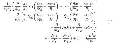
The equations of motion for a curved thick membrane under the action of external forces can be found in Reddy [3] p. 421:

The above equation is described in a curvilinear coordinate system. x₁ and x₁ represent curved coordinates which follow the surface. N₁₁ and N₁₁ are the normal (membrane) forces per unit length. N₁₂ represents the shear force parallel to the curved surface and Q₁ and Q₂ represent the shear forces normal to curved surface. R₁ and R₂ are the curvature radii and f₃ is the external force acting normal to the plane. u₁ and u₂ are the displacements parallel to the curved surface and $w$ is the displacement normal to the curved surface. I₀ = &rho h is the mass per unit surface. a₁ and a₂ are the scale factors (see e.g. https://mathworld.wolfram.com/ScaleFactor.html).

In our case we want only to consider the effect of the pressure on the membrane motion. Since the pressure always acts in surface normal direction, it reasonable to assume that the displacements parallel to the surface u₁ and u₂ can be neglected. For thin membranes the transverse shear forces Q₁ and Q₂ are usually set to zero (see \cite{reddy2006theory}). Since the pressure acts in surface normal direction is it also reasonable to assume that the membrane is not rotated parallel to the surface and hence also the shear force N₁₂ can be neglected. With this assumption we obtain the following equation:

The first term in the above equation can be identified as the Laplacian in curvilinear grids (see e.g. http://sites.science.oregonstate.edu/~corinne/COURSES/ph461/laplacian.pdf). Therefore we can write down the above equation as:

The matrix N is defined as:

It evident that the term the first term on the left of the above equation can be seen as an diffusion equation with an anisotropic diffusion (see also [1])

The constitutive relations for a thin shell can be found in [3] p. 429:

&epsilon₁₁, &epsilon₂₂ and &epsilon₁₂ are the longitudinal, the lateral and the shear strain, respectively. The constant A is defined as follows:

E is the Young modolus, h is the thickness of the membrane and &nu is the Poisson ratio.

Implementation

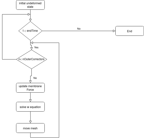
The algorithm proposed to solve the non-linear equation for the membrane (remember that the membrane force N is a function of the displacement w normal to the surface) is a simple predictor corrector algorithm. It is shown in the figure below. We start from the initial (undeformed) state. After that the time marching is started until the end time is reached. Within each time step the membrane equation can be solved several times by specifying a number of nOuterCorrectors in the fvSolution dictionary grater than 1. The solution procedure for the membrane equation is the following: 1) Update the membrane force: The membrane force depends on how much neighboring face centers are displaced relative to the initial stage. The magnitude of the displacement is retrieved from geometrical information, i.e. it is calculated from the distance between face centers adjacent to an edge and distances between the two points forming an edge. Since the mesh is moved at the end of the loop, the membrane force has to be updated at the beginning in order to retrieve the correct displacements. 2) Solve the membrane equation with the updated membrane force to get the displacement in surface normal direction w. 3) Move the mesh in the direction of the undeformed (initial) surface normal by the amount w calculated from the solution of the membrane equation. The three steps are repeated the number of times specified by the user in order to get a better estimation for the membrane force. Note that the flag MeshOuterCorrectors should be set to yes in the fvSolution dictionary in order to allow the mesh to move during the sub iterations within a time step. Otherwise the membrane force will not be updated during the sub iterations.

After having described the algorithm as a whole, we start with the description implementation of our equation with the anisotropic diffusion equation. As we know OpenFOAM uses a finite volume or in our case a finite area method to discretize the governing equation. If we integrate the anisotropic diffusion equation over the finite area and apply the Gauss-Green theorem we get:

In the above equation $dA$ represent the differential area element a $\mathbf{E}$ is the edge vector (in a finite volume discretization it corresponds to the surface area vector). The summation index $e$ means that we have to sum over the edges of the finite area element. With an additional manipulation of the above equation (see also \cite{moukalled2016} p. 255) we obtain the final discretized equation:

It is evident that the term N^T * E represent the projection of the membrane force in direction of the edge vector E

The anisotropic diffusion equation is implemented as follows:

fam::laplacian(normalForcef_, w_)

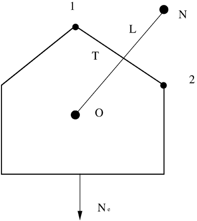
The edgeScalarField normalForcef_ represent the projection of the membrane force vector in direction of the edge vector E. In order to understand the current implementation, it is useful to have a look at the following figure. It represent a general polygonal cell. The cell consists in the cell center (labeled as O) and various neighbors (labeled as N). The distance between the owner cell center and the neighbor cell center is labeled as L. The length of the edge delimited by the points 1 and 2 is labeled as T. N_e represents the projection of the membrane force in direction normal to the cell edge.

In the following we assume that the vectors connecting two adjacent cell centers and the edge of the cell bounding this two cells are normal to each other. This will be true for high quality meshes. For the latter orthonormal system, we can use the constitutive relation to obtain an expression for N_e:

e_e is the strain normal to the edge and e_t is the strain parallel to the edge. The stain e_t can be approximated as:

T represents the length of the edge in the deformed and T₀ in the undeformed (initial) state. The Implementation of this relation looks like:

edgeScalarField ett("ett",(regionMesh().magLe() - initialEdgeLength_) / initialEdgeLength_ );

The edgeScalarField initialEdgeLength_ is the initial edge length and is calculated by the constructor if it not present on the hard drive.

The stain e_e can be approximated as:

L represents the distance between two adjacent cell centers in the deformed and L₀ in the undeformed (initial) state.

The Implementation of this relation looks like the following code snippet for the internal field:

   label edgeCounter = 0;
   
   forAll(ess,edgeI)
   {
    
       vector ownCenter (regionMesh().areaCentres()[regionMesh().edgeOwner()[edgeI]]);
       vector neiCenter (regionMesh().areaCentres()[regionMesh().edgeNeighbour()[edgeI]]);
       scalar distance (mag(ownCenter - neiCenter));
       ess[edgeI] = (distance - initialFaceCenterDistance_[edgeI]) / (initialFaceCenterDistance_[edgeI] + SMALL);
       edgeCounter += 1;        
   }
   

The edgeScalarField initialFaceCenterDistance_ is the initial distance between the face centers of two neighboring finite area cells. It is calculated by the constructor if it is not present on the hard drive.

The treatment of the boundary fields looks like the following code snippet:

  
   auto& bfld = ess.boundaryFieldRef();
   const auto& infc = initialFaceCenterDistance_.boundaryFieldRef();
   

   forAll(bfld, patchi)
   {
       forAll(bfld[patchi],edgeI)
       {
           vector ownCenter (regionMesh().areaCentres()[regionMesh().edgeOwner()[edgeCounter]]);
           vector edgeCenter (regionMesh().edgeCentres().boundaryField()[patchi][edgeI]);
           scalar distance (mag(ownCenter - edgeCenter));
           bfld[patchi][edgeI] = (distance - infc[patchi][edgeI]) / (infc[patchi][edgeI] + SMALL);
           edgeCounter += 1;
       }
           
   }

Finally the calculation of the membrane force normal to the edge looks like this:

   normalForcef_ = Ah() * (ess + solid().nu() * ett);  

The whole code to for the calculation of the membrane force normal to the edge is represented in the following:

void linearElasticMembraneModel::updateNormalForce() {

   edgeScalarField ett("ett",(regionMesh().magLe() - initialEdgeLength_) / initialEdgeLength_ );
   edgeScalarField ess("ess", ett);
   label edgeCounter = 0;
   
   forAll(ess,edgeI)
   {
    
       vector ownCenter (regionMesh().areaCentres()[regionMesh().edgeOwner()[edgeI]]);
       vector neiCenter (regionMesh().areaCentres()[regionMesh().edgeNeighbour()[edgeI]]);
       scalar distance (mag(ownCenter - neiCenter));
       ess[edgeI] = (distance - initialFaceCenterDistance_[edgeI]) / (initialFaceCenterDistance_[edgeI] + SMALL);
       edgeCounter += 1;
       
   }
   
   auto& bfld = ess.boundaryFieldRef();
   const auto& infc = initialFaceCenterDistance_.boundaryFieldRef();
   

   forAll(bfld, patchi)
   {
       forAll(bfld[patchi],edgeI)
       {
           vector ownCenter (regionMesh().areaCentres()[regionMesh().edgeOwner()[edgeCounter]]);
           vector edgeCenter (regionMesh().edgeCentres().boundaryField()[patchi][edgeI]);
           scalar distance (mag(ownCenter - edgeCenter));
           bfld[patchi][edgeI] = (distance - infc[patchi][edgeI]) / (infc[patchi][edgeI] + SMALL);
           edgeCounter += 1;
       }
           
   }
   
   normalForcef_ = Ah() * (ess + solid().nu() * ett);
   

}

The next point in this tutorial is how to calculate the external forces $f_3$. In our equations we will consider only the gravity force and the pressure:

The pressure p is taken from the fluid domain. g * n is the scalar product of the gravitational acceleration g and unit normal face vector n. The gravity force is implemented as follows:

    areaScalarField linearElasticMembraneModel::gravityForce()

{

   return regionMesh().faceAreaNormals() & g_ * rho();

}

The last point in the description of the implementation is how we treat the terms: N₁₁/R₁ + N₂₂/R₂. Since the curvatures &kappa₁ = 1/R₁ and &kappa₂ = 1/R₂ we can write down the equations as:

Let's recall that $N_{11}$ and $N_{22}$ are the membrane forces in direction of the curvilinear coordinates &xi₁ and &xi₂. &kappa₁ and &kappa₂ are the corresponding curvatures. The faMesh class offers a build in function which return the face curvature &kappa_f. The curvature of the face is basically calculated by the scalar product of the face normal n_f with the edge integral of the length vector l_eover the face edges divided by the face surface S_f

The same procedure is applied to calculate the influence of the surface curvature on the displacement of the membrane normal to the surface:

void linearElasticMembraneModel::curvatureForce()

{

   areaVectorField kN(fac::edgeIntegrate(regionMesh().edgeLengthCorrection()*regionMesh().Le()*normalForcef_));

   curvatureForce_  = -sign(kN&regionMesh().faceAreaNormals())*mag(kN);

A better estimation for the computation of the term N₁₁ &kappa₁ + N₂₂ &kappa₂ would be to compute the curvature at each cell edge &kappa_e, multiply it with the membrane force normal to the corresponding edge $N_e$ and sum the this product over the cell edges. Unfortunately I did not find yet a working implementation for this.

Test cases

Cylinder with internal pressure

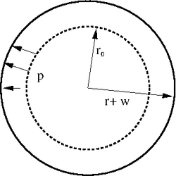
The next figures shows a sketch of the first test case. This first test case consists in a circular cylinder with an undeformed radius r₀ = 1 m, a Young modolus of E = 2.1 x 10⁶ N/m² and a thickness of h = 3 x 10^-4 m. The undeformed cylinder is subject to an internal pressure of p = 70Pa in radial direction. The ends of the cylinder a free to move (i.e. they are not clamped). For this configuration an analytical solution exists (see [4] p. 475): w = p r₀²/(E h) = 0.111 m.

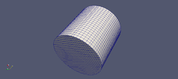
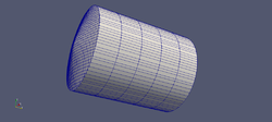
The mesh topography is shown in the next figure. In order to generate the mesh for we use blockMes in order to get a hexaedral mesh and after the we use snappyHexmesh in order to obtain the cylindrical shape. The results of four different meshes are compared in order to check if the can get a grid independent solution. The meshes differ in the number of cells used in radial and circumferential direction. The number of cells in axial direction was kept unchanged. The figure below shows the mesh with approximately 50 cells in circumferential direction. The four meshes compared had approximately N = 25, 50, 100 and 200 cells in circumferential direction.

The results of the mesh sensitivity study is shown in the table below. It is evident that we could not reach a grid independent solution with the maximum number of N = 200 cells in circumferential direction. The reason is probable that the curvature should be computed as function of the direction. In our simplification we used an average curvature for each finite area element. The agreement with the analytical solution is reasonable.

Circular membrane subject to constant pressure

The second test case consists in a circular membrane with a radius r = 0.08$ m, a Young modolus of E = 2.1 x 10⁶ N/m² and a thickness of h = 3.4 x 10^-4 m. The pressure acts in this case normal to surface in y-direction. The same case was also studied by [2] experimentally and numerically. [2] measured and simulated the displacement of the membrane for different pressures. For the evaluation of our model we took the maximum and minimum pressure studied by [2]: p = 70 and p = 230 Pa. The membrane is clamped at the outer border. A sketch of the configuration is provided below.

In order to check if we can reach mesh independent results, we simulate two meshes with around 20 and 40 cells in radial direction. The coarser mesh in the deformed stage is shown in the figure below.

The result obtained for the current test case are shown in the figure below. The left figure shows the comparison with the experiments of [[2]. The first observation is that the two meshes deliver very similar results. This means that we could obtain fairly mesh independent results. The second observation is that the agreement with the experiment is acceptable especially keeping in mind the simplicity of the model. The maximum displacement is reproduce quite well. We can observe that the experiment show profile which is more curved respect to the current results. The reason is probably that we displace the membrane only in the initially undeformed direction.

Lessons learned

• By making a few assumption we could derive a simple expression which describes the non linear membrane displacement

• When simplifying equation we need always the check the range of applicability by careful designed test cases

• We could use geometrical relations stored in the mesh class to derive an expression for the membrane force

• The results can probably be improved by implement an anisotropic expression for the curvature and displace the mesh in direction of the actual normal instead of the undeformed normal

• The finite area method is a very elegant way to couple 2D physical models acting as boundary conditions for the 3D computational domain

References

[1] Fadl Moukalled, L Mangani, Marwan Darwish, et al. The finite volume method in computational fluid dynamics, volume 113. Springer, 2016.

[2] Draga Pihler-Puzović, Anne Juel, Gunnar G Peng, John R Lister, and Matthias Heil. Displacement flows under elastic membranes. part 1. ex- periments and direct numerical simulations. Journal of Fluid Mechanics, 784:487–511, 2015.

[3] Junuthula Narasimha Reddy. Theory and analysis of elastic plates and shells. CRC press, 2006.

[4] Stephen Timoshenko, Sergius Woinowsky-Krieger, et al. Theory of plates and shells, volume 2. McGraw-hill New York, 1959.